Scaling Vector Search with pgvector

Before you sign a contract for a specialized vector database like Pinecone, Weaviate, or Qdrant for your RAG pipeline, take a hard look at your primary database. If your stack already runs PostgreSQL, you probably do not need a dedicated vector database.

Spinning up a standalone vector database means managing two sources of truth, writing dual-write synchronization scripts, and dealing with eventual consistency nightmares whenever users delete or update records.

With the pgvector extension, your embeddings live directly alongside your relational tables: sharing the same ACID guarantees, automatic backups, and seamless hybrid SQL joins.

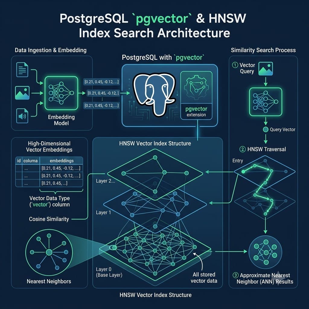
Here is how vector search works in RAG pipelines, how to configure pgvector, build HNSW indexes that scale past a million embeddings, and perform fast cosine similarity searches without leaving Postgres.

Where standalone vector databases fall down

Dedicated vector databases like Pinecone, Milvus, or Qdrant are solid tools, but introducing one into your stack means:

1. You maintain a secondary database and write dual-sync pipelines.
2. If a user deletes an account or edits an article in Postgres, you must coordinate a distributed delete/update in the vector store.
3. Permission checks (WHERE org_id = $1) turn into an awkward pre-filtering or two-step query dance.

With pgvector, your embeddings live right in your primary database. An insert is an ACID transaction. A delete cleans up both the row and its vector simultaneously.

Setting Up pgvector

Getting started with pgvector is highly straightforward. If you are using a modern managed PostgreSQL provider (such as AWS RDS, Supabase, Google Cloud SQL, or Neon), pgvector is almost certainly already supported and merely needs to be enabled.

If you are running PostgreSQL locally or on a custom server, you can compile and install it from the source. Once the binary is installed on your server, enable the extension in your database by running the following SQL command:

-- Enable the pgvector extension in your database
CREATE EXTENSION IF NOT EXISTS vector;

With the extension successfully enabled, you can now utilize the new vector data type. Let's create a table to store our text document chunks and their corresponding embeddings. For example, if we are using OpenAI's standard embeddings, the dimensions typically equal 1536.

-- Create a table to store documents, metadata, and their vector embeddings
CREATE TABLE documents (
    id bigserial PRIMARY KEY,
    content text NOT NULL,
    metadata jsonb,
    -- Store a vector array with precisely 1536 dimensions
    embedding vector(1536)
);

Inserting data into this table is just as simple as inserting into any other Postgres table. You simply provide the vector as a formatted string or a standard array from your application code:

-- Insert a sample document and its semantic embedding
INSERT INTO documents (content, metadata, embedding)
VALUES (
    'Vector search enables semantic matching based on meaning, rather than keywords.',
    '{"author": "Jane Doe", "category": "AI", "tenant_id": 101}',
    '[0.012, -0.045, 0.088, ..., 0.011]'
);

Performing Cosine Similarity Search

To find the most relevant documents for a given query, we must first convert the user's plain-text query into an embedding using the exact same embedding model, and then search the database for the closest vectors. pgvector supports several distance metrics natively, including Euclidean distance (<->), inner product (<#>), and cosine distance (<=>).

For most modern LLM embeddings (which are often normalized by the provider), cosine distance is the standard and recommended metric. Here is how you can perform a K-Nearest Neighbors (KNN) search to rapidly find the top 5 most semantically similar documents:

-- Find the 5 most semantically similar documents to a user's query vector
SELECT 
    id, 
    content, 
    -- Calculate cosine similarity by subtracting distance from 1
    1 - (embedding <=> '[0.015, -0.042, 0.091, ..., 0.021]') AS similarity_score
FROM documents
ORDER BY embedding <=> '[0.015, -0.042, 0.091, ..., 0.021]'
LIMIT 5;

Notice that the custom operator <=> computes the cosine distance. Because cosine similarity is mathematically defined as 1 - cosine_distance, we simply subtract the distance from 1 in our SELECT clause to retrieve an intuitive similarity score.

Scaling with HNSW Indexes

A standard KNN query as shown above performs a sequential scan, examining every single row in the table to calculate the exact distance. While this Exact Nearest Neighbor (ENN) approach guarantees perfect accuracy, it becomes incredibly slow as your dataset grows into the hundreds of thousands or millions of rows.

To scale vector search to enterprise levels, we must use Approximate Nearest Neighbor (ANN) algorithms. These algorithms trade a tiny, often imperceptible bit of accuracy (recall) for massive, logarithmic performance gains. Starting in version 0.5.0, pgvector introduced robust support for HNSW (Hierarchical Navigable Small World) indexes: widely considered the gold standard algorithm for vector search today.

HNSW builds a multi-layered graph where each node represents a vector. Searches start at the highest, sparsest layer, making large jumps across the vector space to quickly narrow down the neighborhood, and progressively drill down to lower, denser layers for fine-grained navigation.

Here is how you create an HNSW index in pgvector, explicitly optimized for cosine distance:

-- Create an HNSW index optimized for cosine distance calculations
CREATE INDEX documents_embedding_hnsw_idx 
ON documents 
USING hnsw (embedding vector_cosine_ops)
WITH (m = 16, ef_construction = 64);

Performance Tuning: m and ef_construction

The HNSW index creation command accepts two critical parameters that allow you to precisely tune the tradeoff between build time, memory footprint, and search recall:

• m: The maximum number of bidirectional links created for each element during graph construction. A higher m (e.g., 32, 64, or even 96) improves recall for high-dimensional data (like 1536-dimensional vectors) but significantly increases the index size on disk and RAM, as well as the build time. The default is 16, but 64 is often recommended for heavy production workloads.
• ef_construction: The size of the dynamic candidate list used when building the index. Increasing this value (e.g., to 128, 256, or 512) results in a meticulously constructed, higher-quality graph and better recall, at the explicit cost of significantly longer index creation times. It only impacts index build time, not query time.

Additionally, during query execution, you can dynamically tune ef_search for the current transaction or session to control the number of candidates considered during the search phase. Higher values increase recall but slightly reduce search speed.

-- Adjust ef_search for the current session to prioritize recall (default is 40)
SET hnsw.ef_search = 100;

Hybrid Search: The Ultimate Postgres Advantage

One of the most compelling reasons to use pgvector over a standalone vector database is the ability to perform complex hybrid searches. You can seamlessly and transactionally combine vector similarity with traditional SQL filters and joins. For instance, you can effortlessly filter documents by a specific author, tenant ID, or a strict date range before ranking the remaining subset by semantic relevance.

SELECT 
    content,
    metadata->>'author' AS author,
    1 - (embedding <=> '[0.015, -0.042, 0.091, ..., 0.021]') AS similarity
FROM documents
WHERE metadata->>'category' = 'AI'
  AND (metadata->>'tenant_id')::int = 101
ORDER BY embedding <=> '[0.015, -0.042, 0.091, ..., 0.021]'
LIMIT 5;

If your standard columns are properly indexed (e.g., using B-Tree or GIN indexes on the metadata JSONB column), PostgreSQL's sophisticated query planner can aggressively filter the dataset first, applying the expensive vector search only to the relevant, highly targeted subset. This is notoriously difficult, heavily latent, and error-prone to achieve efficiently in split architectures where relational metadata lives in Postgres and vectors live completely isolated in a separate database system.

Operational rules of thumb before you scale

pgvector with HNSW handles millions of vectors easily, but keep these practical limits in mind:

1. RAM constraints: HNSW indexes must fit in memory. 1 million 1536-dimensional vectors with m = 32 will consume roughly 2.5GB to 3GB of RAM for the index alone. If your index spills to disk, query latency jumps from 8ms to 200ms+. Size your shared_buffers and RAM accordingly.
2. Read replicas: Vector search is CPU and memory intensive. Once search traffic climbs, spin up a dedicated Postgres read replica just for vector queries so you never starve your primary OLTP connection pool.
3. Filtered ANN recall: If you run heavy multi-tenant filters (WHERE tenant_id = $1), consider partial HNSW indexes per tenant or pgvector 0.7's iterative index scans to prevent recall degradation.

If you have under 10 million vectors, start with Postgres. It keeps your stack simple and your operational overhead near zero.

You Might Also Like

• AI Coding Assistants: Best Practices for 2026
• Cursor vs Claude Code: Which ai Coding Tool Actually Wins in 2026?
• How I Actually Use ChatGPT, Claude, and Gemini for Development Work
• Cursor IDE Advanced Features for Pragmatic Engineers: MCP, Rules, and Agents in 2026