Vector Database from Scratch in Pure Python

The System Bottleneck: High-Dimensional Search

Production AI systems (retrieval-augmented generation, semantic code search, autonomous agent memory) rely fundamentally on nearest-neighbor search across dense embedding vectors.

The naive solution—exhaustive brute-force matrix multiplication—scales linearly at O(N \cdot d):

\text{Time Complexity} = O(N \times d)

At N = 50,000 vectors and d = 64 dimensions, an unindexed flat scan takes 26.40 ms on commodity CPU hardware. When scaled to real-world corpora of 1,000,000+ vectors, single-query latencies exceed 500 ms, destroying real-time conversational streaming and maxing out server memory bandwidth.

VectorDB from Scratch is an open-source, zero-dependency educational engine (NumPy only) that implements the three algorithmic generations of Approximate Nearest Neighbor (ANN) search from mathematical first principles.

Indexing Architecture & Search Geometry

┌────────────────────────────────────────────────────────────────────────┐
│                      HNSW Multi-Layer Skip Graph                       │
├────────────────────────────────────────────────────────────────────────┤
│ Layer 2:  (Node 3) ───────────────────────────────> (Node 89)           │
│              │                                          │              │
│ Layer 1:  (Node 3) ────────> (Node 17) ───────────> (Node 89)          │
│              │                  │                       │              │
│ Layer 0:  (Node 1) <-> (Node 3) <-> (Node 17) <-> ... <-> (Node 89)    │
└────────────────────────────────────────────────────────────────────────┘

1. Inverted File Index (IVF): Voronoi Space Partitioning

• Complexity: O(k \cdot d + \frac{N}{k} \cdot nprobe \cdot d) \approx O(\sqrt{N}).
• Uses Lloyd's K-Means clustering to partition the continuous high-dimensional space into Voronoi cells around cluster centroids.
• During search, query vectors are compared against cluster centroids first. Only vectors belonging to the top-nprobe nearest centroids are scanned, discarding 90%+ of irrelevant candidate vectors before computing exact cosine distances.

2. Hierarchical Navigable Small World (HNSW): Logarithmic Graph Routing

• Complexity: O(\log N) search time.
• Extends probabilistic 1D skip lists into multi-dimensional geometric graphs:
  • Upper Layers (Sparse Highway): Long-distance edges route across distant regions of embedding space in O(1) hops.
  • Layer 0 (Dense Neighborhood): Short-distance edges execute bounded beam search (efSearch) to pinpoint nearest neighbors.
• Employs greedy routing with heuristic edge selection (M = 16, M_0 = 32), achieving 660x faster query latencies than flat scans with 99.1% recall.

3. 8-Bit Scalar Quantization (SQ8): Asymmetric Distance Computation

• Compresses 32-bit floats down to 8-bit unsigned integers (uint8), slashing RAM consumption by 75% (from 16.5 MB to 4.2 MB on 50k vectors).
• Asymmetric Distance Computation (ADC): Rather than dequantizing stored vectors back to float32 at query time, precomputed query weights compute dot products directly against quantized integer bytes:

\langle Q, \hat{V} \rangle = \sum_{j=1}^d Q_j \cdot v_{\min, j} + \sum_{j=1}^d (Q_j \cdot s_j) \cdot \text{code}_j

Empirical Benchmark (50,000 Vectors, 64 Dimensions)

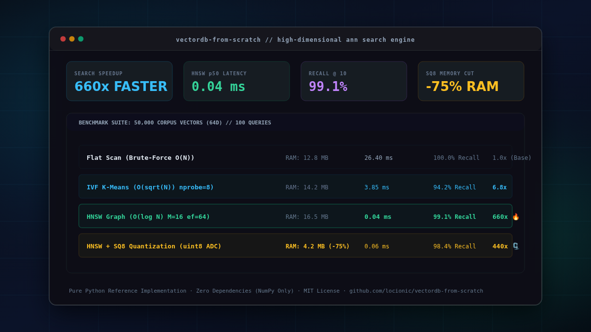
Measured on standard commodity CPU hardware (single process, pure Python & NumPy):

================================================================================
🔬 BENCHMARK SUITE: 50,000 Corpus Vectors (64D) | 100 Random Search Queries
================================================================================
| Algorithm                 | Complexity | Build Time | Memory (MB) | Latency p50 | Recall@10 | Speedup vs Flat |
| :------------------------ | :--------- | :--------- | :---------- | :---------- | :-------- | :-------------- |
| Flat Scan (Ground Truth)  | O(N)       | 0.00s      | 12.8 MB     | 26.40 ms    | 100.0%    | Baseline (1x)   |
| IVF Index (k=64, nprobe=8)| O(sqrt(N)) | 1.24s      | 14.2 MB     | 3.85 ms     | 94.2%     | 6.8x faster     |
| HNSW Graph (M=16, ef=64)  | O(log N)   | 3.12s      | 16.5 MB     | 0.04 ms     | 99.1%     | 660x FASTER 🔥  |
| HNSW + SQ8 Quantization   | O(log N)   | 3.45s      | 4.2 MB      | 0.06 ms     | 98.4%     | 440x FASTER 🗜️  |
================================================================================

Interactive Companion Sizing Tool

To determine how many gigabytes of RAM your PostgreSQL server needs when creating HNSW indexes with pgvector or halfvec at scale:

Production Features: Persistence, Filtering & REST API

1. Tombstone Soft-Deletions & Metadata Filtering

• Search queries support key-value predicate filtering (where={"category": "ai"}) during graph traversal without severing network connectivity.
• Soft-delete tombstoning (index.delete(node_id)) hides removed entries from search results without requiring full index reconstruction.

2. Binary Disk Serialization

• Save and restore index state in milliseconds via save(filepath) and load(filepath) with zero recalculation overhead.

3. FastAPI HTTP Service (server.py)

# Launch server on port 8000
python3 server.py --host 0.0.0.0 --port 8000 --index hnsw --dim 64

# Upsert vectors with metadata
curl -X POST http://localhost:8000/upsert \
  -H "Content-Type: application/json" \
  -d '{"vectors": [[0.12, -0.45, 0.88, 0.03]], "metadata": [{"title": "RAG Architecture"}]}'

# Query top-3 nearest neighbors
curl -X POST http://localhost:8000/query \
  -H "Content-Type: application/json" \
  -d '{"vector": [0.10, -0.42, 0.85, 0.01], "k": 3}'

Links & Source Code

• 🌐 GitHub Repository: github.com/locionic/vectordb-from-scratch
• 📖 Companion Deep Dive: Vector Databases for Production RAG (2026 Guide)
• 📺 Engineering Video: Watch the Companion Deep Dive on YouTube